🎓How I Study AIHISA
📖Read
📄Papers📰Blogs🎬Courses
💡Learn
🛤️Paths📚Topics💡Concepts🎴Shorts
🎯Practice
📝Daily Log🎯Prompts🧠Review
SearchSettings
Chapter 4: Matrix multiplication as composition | Essence of Linear Algebra | How I Study AI
📚 선형대수학의 본질5 / 12
PrevNext
Chapter 4: Matrix multiplication as composition | Essence of Linear Algebra
Watch on YouTube

Chapter 4: Matrix multiplication as composition | Essence of Linear Algebra

Beginner
3Blue1Brown Korean
AI BasicsYouTube

Key Summary

  • •This lesson shows a new way to see matrix multiplication: as doing one geometric change to space and then another. Instead of thinking of matrices as number grids, you think of them as machines that move every vector to a new place. When you do two moves in a row, that is called composition, and it is exactly what matrix multiplication represents. The big idea is that one single matrix can capture the effect of doing two transformations in sequence.
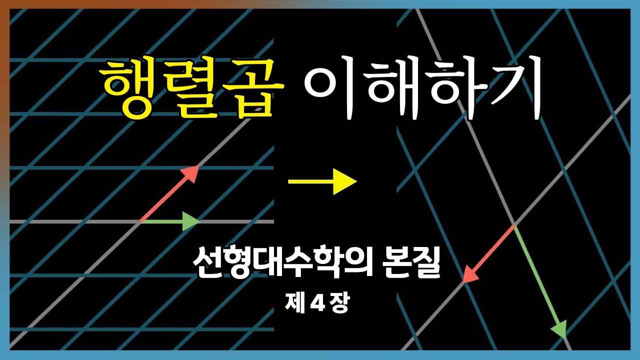
  • •The instructor uses the 2D unit vectors, often called i-hat and j-hat, as the anchors for understanding. A matrix tells you where those two basis arrows go; its columns are the new positions of those arrows. If you know what happens to these two arrows, you know what happens to every vector. This makes it very easy to compute the matrix for a combined transformation.
  • •Order matters a lot: the right-hand matrix acts first, and the left-hand matrix acts second. So if you want to describe “do f, then do g,” the product you write is B times A, not A times B. Switching the order usually gives a different result, because the two transformations interact differently. This non-commutativity is a key takeaway.
  • •You can compute the columns of the product matrix by taking linear combinations of the left matrix's columns using the entries from the right matrix's columns. Practically, you focus on where the first basis vector goes after the first transformation, then apply the second transformation to that result. You repeat for the second basis vector. These two outputs become the two columns of the product.
  • •Thinking visually helps: imagine first stretching and shearing the whole plane, then applying another stretch or shear. The combined effect can be summarized by a single matrix that sends the original basis arrows to their final positions. This view turns matrix multiplication into an easy-to-picture story. It also explains why multiplication is defined exactly the way it is.

Why This Lecture Matters

Seeing matrix multiplication as composition changes the experience from memorizing steps to understanding. It is useful for students in algebra, physics, computer graphics, robotics, and data science who work with transformations. Problems like chaining camera transforms, simulating motions, or combining filters all rely on composing multiple linear steps; recognizing that the product matrix represents the full chain makes these tasks reliable and efficient. In real projects, it helps you design complex effects by breaking them into simpler, testable parts—each with its own matrix—then multiplying in the correct order. This skill boosts career development by turning you into someone who not only computes answers but also explains and predicts outcomes, which is valuable in technical roles. In today’s industry, linear algebra underlies machine learning models, 3D engines, and control systems; understanding composition gives you a clean mental model to build, debug, and optimize pipelines of transformations.

Lecture Summary

Tap terms for definitions

01Overview

This lesson teaches you to see matrix multiplication as composition of transformations: doing one geometric change to space and then doing another. Instead of viewing matrices as just grids of numbers, you see them as machines that move every vector to a new place. In two dimensions, a 2×22×22×2 matrix moves the entire plane; in three dimensions, a 3×33×33×3 matrix moves all of 3D space. When you apply two such machines one after the other, the whole result can still be described by one single matrix. This is exactly what matrix multiplication is: a compact way to represent “do this change, then that change.”

The core idea centers on the standard basis vectors, often called i-hat and j-hat. Think of these as the two basic arrows that define the x and y directions. A matrix tells you where those arrows go; its two columns are exactly the new positions of those arrows after the transformation. If you know where these two arrows land, you know how any vector will move, because any vector can be built as some amount of i-hat plus some amount of j-hat. This turns multiplication into a very visual, understandable process.

The audience for this lesson includes beginners who know basic vector ideas and want to understand matrix multiplication deeply, as well as intermediate learners who have computed many products but want the geometric meaning. You should know what vectors are, what a linear transformation is in simple terms (a rule that scales, rotates, or shears but keeps straight lines straight), and how a matrix times a vector gives a new vector. With that, you’re ready to see why the multiplication rule is defined the way it is and how to compute products confidently.

After completing this lesson, you will be able to: describe a matrix as a transformation of space; explain why multiplying matrices represents doing one transformation after another; compute product matrices column by column using the images of basis vectors; and avoid common mistakes, especially getting the order backward. You will also be able to connect the arithmetic of matrix multiplication to its geometric meaning, so every number in the product has a clear purpose.

The lesson is structured as follows. First, it reframes matrices as transformations that move the whole space and shows how the columns encode where the basis vectors go. Next, it explains composition: doing transformation f, then transformation g, and writing the combined effect as a single matrix. It shows a concrete 2D example with specific images for i-hat and j-hat under each transformation and computes the final matrix by following i-hat and j-hat through the two-step process. Then it connects this to the standard multiplication rule, showing that each column of the product is a linear combination of the left matrix’s columns with weights from the right matrix’s columns. Finally, it stresses the importance of order and summarizes how to think of matrix multiplication going forward: always as “first this change, then that change,” with the right-hand matrix acting first and the left-hand matrix acting second.

Key Takeaways

  • ✓Always think of a matrix as a space-moving machine, not just a number grid. Picture where the x- and y-unit arrows go; those are the columns. If you can see those two images, you can predict the matrix’s effect on any vector. This mental model replaces blind memorization with clear insight.
  • ✓Matrix multiplication is composition: the right-hand matrix acts first. If you want to do A then B, form BA. Keep repeating “right first, left second” until it becomes automatic. This simple habit prevents many mistakes.
  • ✓Build product columns by applying the left matrix to the right matrix’s columns. Start with the first column of the right matrix, transform it, and that’s your first product column. Repeat for the second column. This is the fastest way to get the product without confusion.
  • ✓Use linear combinations to compute matrix–vector outputs. Write the input as x of i-hat plus y of j-hat, then make the same mix of the matrix’s columns. This approach is quick, reliable, and deeply meaningful. It also makes product computations straightforward.
  • ✓Check your work visually by sketching the unit square. Track where (1, 0) and (0, 1) go through each step. The final positions should match your product’s columns. If not, re-check your order or arithmetic.
  • ✓Remember that order matters and products usually don’t commute. Swapping factors changes the geometry the second step sees. If results look odd, ask if you reversed the order. Correcting the order often fixes the issue.
  • ✓Translate between the row–column arithmetic and the column picture. Each entry is a dot product, but each column is also a transformed basis vector. Both views should agree; if they don’t, an error hides in your calculations. Use one to check the other.

Glossary

Linear transformation

A rule that moves vectors so that straight lines stay straight and the origin stays fixed. It can stretch, shrink, rotate, or shear the space. In 2D, it moves the whole plane in a consistent way. It is exactly what a matrix represents. Every output depends on the input in a proportional and add-on-friendly way.

Matrix

A rectangular grid of numbers that represents a linear transformation. In 2D, it has two columns that show where the x- and y-unit vectors go. It turns input vectors into output vectors by a special multiplication rule. Each entry affects how much of each input direction contributes to each output direction.

Basis vector

A simple building-block vector used to describe all other vectors. In 2D, the standard basis vectors are one step in x and one step in y. Any vector can be written as some amount of these. A matrix shows where these basic arrows go.

i-hat (unit x vector)

The unit vector pointing one step along the x-axis. It is one of the two standard basis vectors in 2D. Matrices tell you where this arrow goes by looking at their first column. Tracking it helps build product matrices.

#matrix multiplication#composition#linear transformation#basis vectors#column picture#row-by-column rule#non-commutative#matrix-vector multiplication#2x2 matrix#geometric intuition#linear combination#standard basis#order of operations#i-hat j-hat#columns as images#unit square#product columns#right-to-left rule#dot product
Version: 1
•
The example in the lesson maps i-hat to (1, −2) and j-hat to (3, 0) for the first transformation. The second one maps i-hat to (0, 1) and j-hat to (2, 2). Applying the second after the first sends i-hat to (−4, −3) and j-hat to (0, 3). Those two results form the columns of the final product matrix.
  • •Another way to compute the first column of the product is to write the image of i-hat after the first transformation as a mix of the second matrix’s columns. The numbers used in that mix are exactly the entries from the first matrix’s first column. Do the same with the second column. This matches the usual arithmetic rule for multiplication but now it has a clear meaning.
  • •Vectors can be seen as instructions that say “take this much of i-hat and that much of j-hat.” A matrix uses those instructions to build the output as the same combination of its own columns. This is why columns matter so much: they are the building blocks the matrix uses. Understanding this makes matrix–vector multiplication and matrix–matrix multiplication feel natural.
  • •Composition is the reason the product of two transformations is still a transformation of the same kind. This keeps everything neat: you can stack many steps and still describe them with just one matrix. It also makes it easy to plan complex effects by breaking them into simple steps. Each step is a matrix, and the final outcome is their product.
  • •The rule “right first, left second” matches how function composition is written in math. It also matches how you would apply a sequence of actions in time. This rule prevents confusion when building chains of transformations. Remembering it avoids many mistakes.
  • •Non-commutativity shows up clearly with geometric pictures: shear then rotate is different from rotate then shear. Even with simple 2D shears and stretches, reversing order changes the outcome. That’s why AB rarely equals BA. Being mindful of order helps you debug and predict results.
  • •Ultimately, matrix multiplication is not an arbitrary set of steps. It is the only way that makes the product matrix correctly capture “do one change, then another,” using the column-as-image-of-basis idea. Once you see it this way, the arithmetic becomes a natural consequence of the geometry. You can compute confidently and understand what every number means.
  • 02Key Concepts

    • 01

      Matrix as transformation: Definition: A matrix is a rule that moves every vector in space to a new place in a straight-line-preserving way. Analogy: It’s like a machine that stretches, squishes, or slants the whole sheet of paper. Technical: In 2D, the two columns show where the original x- and y-direction arrows land. Why it matters: If you know where those two arrows go, you know the whole transformation. Example: A matrix with first column (1, −2) and second column (3, 0) sends the x-arrow to (1, −2) and the y-arrow to (3, 0), so any vector built from those arrows will be moved accordingly.

    • 02

      Composition of transformations: Definition: Composition means doing one transformation and then another right after it. Analogy: Like first putting a photo through a stretch filter, then applying a tilt filter. Technical: If the first transformation is f and the second is g, the composition is g after f, and it is itself a transformation. Why it matters: You can string steps together but still describe it with a single matrix. Example: If step one turns i-hat into (1, −2) and j-hat into (3, 0), and step two maps i-hat to (0, 1) and j-hat to (2, 2), then doing step two after step one sends i-hat to (−4, −3) and j-hat to (0, 3).

    • 03

      Matrix multiplication equals composition: Definition: The product of two matrices is the single matrix that does first the right-hand transformation and then the left-hand one. Analogy: Think of stacking two transparent sheets that each distort a drawing; together they act like one special sheet. Technical: The columns of the product come from applying the left matrix to the columns of the right matrix, one by one. Why it matters: Multiplication is not arbitrary arithmetic; it encodes “do this, then that.” Example: Using the example above, the final matrix has columns (−4, −3) and (0, 3), which is the product of the two given matrices.

    • 04

      Columns as images of basis vectors: Definition: Each column of a matrix is where a basis vector (the simple unit arrow) goes. Analogy: The two columns are like two GPS pins showing where the x- and y-arrows moved. Technical: Any input vector is x of i-hat plus y of j-hat, so the output is x of the first column plus y of the second column. Why it matters: It makes matrix–vector multiplication simple to understand and compute. Example: If a vector is 2 of i-hat plus −1 of j-hat, and the matrix columns are (1, −2) and (3, 0), the output is 2⋅(12·(12⋅(1, −2) + (−1)⋅(31)·(31)⋅(3, 0) = (−1, −4).

    • 05

      Right-to-left order: Definition: In a product of matrices, the right-hand matrix acts first on vectors, then the next to its left, and so on. Analogy: Like dressing: you put on socks before shoes; the socks step is closer to your foot, so it happens first. Technical: Writing “do f, then g” corresponds to multiply by A (for f) and then by B (for g), which is described by BA. Why it matters: Getting the order wrong usually changes the result. Example: Doing a shear then a stretch is generally different from stretching first and then shearing.

    • 06

      Computing product columns: Definition: Each column of the product matrix is the left matrix applied to a column of the right matrix. Analogy: Feed each right-matrix column through the left machine; the outputs become the product’s columns. Technical: Focus on where i-hat goes after the first step, then run that through the second step to get the product’s first column; repeat for j-hat. Why it matters: This avoids confusion and matches the geometric story. Example: If i-hat maps to (1, −2) after step one and the second matrix sends (1, −2) to (−4, −3), then (−4, −3) is the first column of the product.

    • 07

      Linear combination viewpoint: Definition: A linear combination is a sum like a⋅column1a·column1a⋅column1 + b⋅column2b·column2b⋅column2. Analogy: It’s like mixing two paint colors in amounts a and b to get a new color. Technical: To get the product’s first column, combine the left matrix’s columns with weights given by the right matrix’s first column entries; repeat for the second column. Why it matters: This links the usual multiplication rule to a clear meaning. Example: With left columns (0, 1) and (2, 2) and right first column (1, −2), compute 1⋅(01·(01⋅(0, 1) + (−2)⋅(22)·(22)⋅(2, 2) = (−4, −3).

    • 08

      Matrix–vector multiplication meaning: Definition: Multiplying a matrix by a vector builds the output as the same mix of the matrix’s columns as the vector uses for i-hat and j-hat. Analogy: The vector is a recipe, and the matrix’s columns are the ingredients. Technical: If the vector is (x, y), the output is x⋅(firstx·(firstx⋅(first column) + y⋅(secondy·(secondy⋅(second column). Why it matters: This is the building block for understanding matrix–matrix multiplication. Example: If the columns are (1, −2) and (3, 0) and the vector is (2, −1), the result is 2⋅(12·(12⋅(1, −2) + (−1)⋅(31)·(31)⋅(3, 0) = (−1, −4).

    • 09

      Non-commutativity: Definition: In general, swapping the order of two matrices changes the result. Analogy: Brushing your teeth and then drinking orange juice is not the same experience as drinking orange juice and then brushing teeth. Technical: Because each step reshapes space, the second step acts on a different shape when order changes. Why it matters: You must keep track of order to predict outcomes. Example: A horizontal shear followed by a vertical stretch usually differs from a vertical stretch followed by a horizontal shear.

    • 10

      Reading transformation from columns: Definition: You can understand a matrix by reading its columns as the new positions of the x- and y-arrows. Analogy: The columns are like “before and after” photos of the two basic arrows. Technical: Once you know these, you can compute the effect on any vector by linear combination. Why it matters: This gives quick intuition without heavy arithmetic. Example: If the columns are (0, 1) and (2, 2), the x-arrow tips up, and the y-arrow becomes a diagonal pointing to (2, 2), indicating a mix of shear and stretch.

    • 11

      Composing via basis tracking: Definition: To compose two transformations, follow what happens to the basis arrows through both steps. Analogy: Track two tagged birds as they fly through two wind tunnels in sequence. Technical: First apply the right-hand transformation to each basis vector, then apply the left-hand one to those results; put the outcomes as columns of the product. Why it matters: It’s the simplest way to build the product matrix correctly. Example: Track i-hat to (1, −2) then to (−4, −3), and j-hat to (3, 0) then to (0, 3); these two results are the product’s columns.

    • 12

      Why the arithmetic rule makes sense: Definition: The standard row-by-column multiplication rule matches the column-combination story. Analogy: Two different recipes produce the same cake because the steps are just rearrangements of the same mixing. Technical: Each entry in the product is the dot product of a row and a column, which equals the same linear combination built columnwise. Why it matters: Trusting the rule is easier when you see its meaning. Example: Computing the top-left entry by a row–column dot product equals the x-component of the left-applied-to-right-first-column result.

    • 13

      Basis independence of composition: Definition: The composed transformation is well-defined no matter how you choose to compute it; columns just make it easy. Analogy: Whether you navigate by compass or by landmarks, you end up at the same destination if you follow the same path. Technical: Applying the left matrix to each right-matrix column or doing row-by-column multiplication yields the same matrix. Why it matters: Multiple correct methods build confidence and flexibility. Example: Using either method with the given two matrices yields the same columns (−4, −3) and (0, 3).

    • 14

      Visual intuition: Definition: Composition is seeing one global reshape followed by another. Analogy: First flatten the dough in one direction, then slide it sideways; the final shape summarizes both actions. Technical: Linear transformations keep grid lines straight but change their spacing and angle; composition stacks these changes. Why it matters: Pictures help predict how areas, angles, and directions change. Example: You can sketch where the unit square’s corners end up after each step to see the product matrix’s columns.

    • 15

      Common mistake—reversing order: Definition: A frequent error is writing the product in the same order you say the steps. Analogy: Saying “first A then B” and writing AB instead of BA is like reading from left to right when the rule is right to left. Technical: The rightmost matrix acts first on vectors. Why it matters: Reversing order can change answers entirely. Example: If you compute AB instead of BA for the given matrices, you do not get columns (−4, −3) and (0, 3); the result differs.

    • 16

      From vectors to matrices: Definition: Matrix–matrix multiplication is just doing matrix–vector multiplication twice, once for each basis vector. Analogy: Test a machine with two standard test inputs to learn its full behavior. Technical: Feed the right matrix’s first column through the left matrix to get the product’s first column; then do the second column. Why it matters: This reduces matrix multiplication to two familiar vector multiplications in 2D (or n in nD). Example: In 2D, compute two outputs for i-hat and j-hat; in 3D, you’d compute three outputs for the three basis arrows.

    03Technical Details

    Overall architecture/structure of the idea

    1. Matrices as linear transformations
    • A 2×22×22×2 matrix acts on the 2D plane; its two columns are the images of the standard basis vectors, usually written as ı^\hat{\imath}^ and ȷ^\hat{\jmath}^​ (the unit x- and y-arrows). Example: If the columns are (1,−2)(1, -2)(1,−2) and (3,0)(3, 0)(3,0), then ı^\hat{\imath}^ goes to (1,−2)(1, -2)(1,−2) and ȷ^\hat{\jmath}^​ goes to (3,0)(3, 0)(3,0); this means the matrix is (13−20)\begin{pmatrix} 1 & 3 \\ -2 & 0 \end{pmatrix}(1−2​30​) (Example: Using (13−20)\begin{pmatrix} 1 & 3 \\ -2 & 0 \end{pmatrix}(1−2​30​), ı^\hat{\imath}^ maps to (1,−2)(1,-2)(1,−2) and ȷ^\hat{\jmath}^​ maps to (3,0)(3,0)(3,0)). Any vector v\mathbf{v}v in the plane can be written as v=x ı^+y ȷ^\mathbf{v} = x\,\hat{\imath} + y\,\hat{\jmath}v=x^+y^​, so the matrix sends v\mathbf{v}v to xxx times its first column plus yyy times its second column (Example: If v=(2−1)\mathbf{v} = \begin{pmatrix} 2 \\ -1 \end{pmatrix}v=(2−1​) and the columns are (1,−2)(1,-2)(1,−2) and (3,0)(3,0)(3,0), the output is 2⋅(1,−2)+(−1)⋅(3,0)=(−1,−4)2\cdot (1,-2) + (-1)\cdot (3,0) = (-1,-4)2⋅(1,−2)+(−1)⋅(3,0)=(−1,−4)).

    • In coordinates, matrix–vector multiplication is often written as (abcd)(xy)=(ax+bycx+dy)\begin{pmatrix} a & b \\ c & d \end{pmatrix} \begin{pmatrix} x \\ y \end{pmatrix} = \begin{pmatrix} ax + by \\ cx + dy \end{pmatrix}(ac​bd​)(xy​)=(ax+bycx+dy​). Example: With (13−20)(2−1)\begin{pmatrix} 1 & 3 \\ -2 & 0 \end{pmatrix} \begin{pmatrix} 2 \\ -1 \end{pmatrix}(1−2​30​)(2−1​), you get (1⋅2+3⋅(−1)−2⋅2+0⋅(−1))=(−1−4)\begin{pmatrix} 1\cdot 2 + 3\cdot (-1) \\ -2\cdot 2 + 0\cdot (-1) \end{pmatrix} = \begin{pmatrix} -1 \\ -4 \end{pmatrix}(1⋅2+3⋅(−1)−2⋅2+0⋅(−1)​)=(−1−4​).

    1. Composition of transformations and matrix multiplication
    • If fff and ggg are two transformations, the composition “do fff then ggg” is written g∘fg \circ fg∘f. Example: If fff sends ı^\hat{\imath}^ to (1,−2)(1,-2)(1,−2) and ȷ^\hat{\jmath}^​ to (3,0)(3,0)(3,0), and ggg sends ı^\hat{\imath}^ to (0,1)(0,1)(0,1) and ȷ^\hat{\jmath}^​ to (2,2)(2,2)(2,2), then g∘fg \circ fg∘f sends ı^\hat{\imath}^ first to (1,−2)(1,-2)(1,−2), then to (−4,−3)(−4,−3)(−4,−3), and sends ȷ^\hat{\jmath}^​ first to (3,0)(3,0)(3,0), then to (0,3)(0,3)(0,3).

    • If matrices AAA and BBB represent fff and ggg, respectively, the matrix for g∘fg \circ fg∘f is the product BABABA (right first, then left). Example: With A=(13−20)A = \begin{pmatrix} 1 & 3 \\ -2 & 0 \end{pmatrix}A=(1−2​30​) and B=(0212)B = \begin{pmatrix} 0 & 2 \\ 1 & 2 \end{pmatrix}B=(01​22​) (columns (0,1)(0,1)(0,1) and (2,2)(2,2)(2,2)), the product BABABA equals (−40−33)\begin{pmatrix} -4 & 0 \\ -3 & 3 \end{pmatrix}(−4−3​03​) because the columns are (−4,−3)(−4,−3)(−4,−3) and (0,3)(0,3)(0,3).

    • Order matters: In general BA≠ABBA \neq ABBA=AB. Example: Using the same AAA and BBB, compute AB=(13−20)(0212)=(380−4)AB = \begin{pmatrix} 1 & 3 \\ -2 & 0 \end{pmatrix}\begin{pmatrix} 0 & 2 \\ 1 & 2 \end{pmatrix} = \begin{pmatrix} 3 & 8 \\ 0 & -4 \end{pmatrix}AB=(1−2​30​)(01​22​)=(30​8−4​), which is not (−40−33)\begin{pmatrix} -4 & 0 \\ -3 & 3 \end{pmatrix}(−4−3​03​).

    1. Column-wise rule for the product
    • The jjj-th column of BABABA is BBB applied to the jjj-th column of AAA: (BA)col j=B (Acol j)(BA)_{\text{col }j} = B\,(A_{\text{col }j})(BA)col j​=B(Acol j​). Example: For j=1j=1j=1 with Acol 1=(1−2)A_{\text{col }1} = \begin{pmatrix} 1 \\ -2 \end{pmatrix}Acol 1​=(1−2​) and BBB as above, B(1−2)=1⋅(01)+(−2)⋅(22)=(−4−3)B\begin{pmatrix} 1 \\ -2 \end{pmatrix} = 1\cdot \begin{pmatrix}0 \\ 1\end{pmatrix} + (-2)\cdot \begin{pmatrix}2 \\ 2\end{pmatrix} = \begin{pmatrix}-4 \\ -3\end{pmatrix}B(1−2​)=1⋅(01​)+(−2)⋅(22​)=(−4−3​), so the first column of BABABA is (−4−3)\begin{pmatrix}-4 \\ -3\end{pmatrix}(−4−3​).

    • Equivalently, use linear combinations: If Acol 1=(ac)A_{\text{col }1} = \begin{pmatrix} a \\ c \end{pmatrix}Acol 1​=(ac​), then (BA)col 1=a Bcol 1+c Bcol 2(BA)_{\text{col }1} = a\,B_{\text{col }1} + c\,B_{\text{col }2}(BA)col 1​=aBcol 1​+cBcol 2​. Example: With a=1a=1a=1, c=−2c=-2c=−2, Bcol 1=(01)B_{\text{col }1}=\begin{pmatrix}0 \\ 1\end{pmatrix}Bcol 1​=(01​), and Bcol 2=(22)B_{\text{col }2}=\begin{pmatrix}2 \\ 2\end{pmatrix}Bcol 2​=(22​), we get 1⋅(01)+(−2)⋅(22)=(−4−3)1\cdot \begin{pmatrix}0 \\ 1\end{pmatrix} + (-2)\cdot \begin{pmatrix}2 \\ 2\end{pmatrix} = \begin{pmatrix}-4 \\ -3\end{pmatrix}1⋅(01​)+(−2)⋅(22​)=(−4−3​).

    • Repeat for the second column: (BA)col 2=B (Acol 2)(BA)_{\text{col }2} = B\,(A_{\text{col }2})(BA)col 2​=B(Acol 2​). Example: With Acol 2=(30)A_{\text{col }2} = \begin{pmatrix} 3 \\ 0 \end{pmatrix}Acol 2​=(30​), B(30)=3⋅(01)+0⋅(22)=(03)B\begin{pmatrix}3 \\ 0\end{pmatrix} = 3\cdot \begin{pmatrix}0 \\ 1\end{pmatrix} + 0\cdot \begin{pmatrix}2 \\ 2\end{pmatrix} = \begin{pmatrix}0 \\ 3\end{pmatrix}B(30​)=3⋅(01​)+0⋅(22​)=(03​), the second column of BABABA.

    1. Row-by-column rule aligns with the column picture
    • The usual arithmetic rule says (BA)ij=∑kBikAkj(BA)_{ij} = \sum_{k} B_{ik} A_{kj}(BA)ij​=∑k​Bik​Akj​. Example: For BABABA with B=(0212)B=\begin{pmatrix}0 & 2 \\ 1 & 2\end{pmatrix}B=(01​22​) and A=(13−20)A=\begin{pmatrix}1 & 3 \\ -2 & 0\end{pmatrix}A=(1−2​30​), the top-left entry is 0⋅1+2⋅(−2)=−40\cdot 1 + 2\cdot (-2) = -40⋅1+2⋅(−2)=−4, matching the first entry of the first column (−4,−3)(−4,−3)(−4,−3).

    • Geometrically, this computes the components of BBB applied to each column of AAA. Example: The second row, first column entry is 1⋅1+2⋅(−2)=−31\cdot 1 + 2\cdot (-2) = -31⋅1+2⋅(−2)=−3, agreeing with the y-component of B(1−2)=(−4−3)B\begin{pmatrix}1 \\ -2\end{pmatrix} = \begin{pmatrix}-4 \\ -3\end{pmatrix}B(1−2​)=(−4−3​).

    1. How to implement the product step by step (no code needed)
    • Step 1: Identify the matrices AAA (first-applied transformation) and BBB (second-applied). Example: Let A=(13−20)A=\begin{pmatrix}1 & 3 \\ -2 & 0\end{pmatrix}A=(1−2​30​) and B=(0212)B=\begin{pmatrix}0 & 2 \\ 1 & 2\end{pmatrix}B=(01​22​).

    • Step 2: Extract AAA’s columns Acol 1A_{\text{col }1}Acol 1​ and Acol 2A_{\text{col }2}Acol 2​. Example: Acol 1=(1−2)A_{\text{col }1}=\begin{pmatrix}1 \\ -2\end{pmatrix}Acol 1​=(1−2​) and Acol 2=(30)A_{\text{col }2}=\begin{pmatrix}3 \\ 0\end{pmatrix}Acol 2​=(30​).

    • Step 3: Apply BBB to Acol 1A_{\text{col }1}Acol 1​ to get the first column of BABABA. Example: B(1−2)=(−4−3)B\begin{pmatrix}1 \\ -2\end{pmatrix}=\begin{pmatrix}-4 \\ -3\end{pmatrix}B(1−2​)=(−4−3​), so (BA)col 1=(−4−3)(BA)_{\text{col }1}=\begin{pmatrix}-4 \\ -3\end{pmatrix}(BA)col 1​=(−4−3​).

    • Step 4: Apply BBB to Acol 2A_{\text{col }2}Acol 2​ to get the second column of BABABA. Example: B(30)=(03)B\begin{pmatrix}3 \\ 0\end{pmatrix}=\begin{pmatrix}0 \\ 3\end{pmatrix}B(30​)=(03​), so (BA)col 2=(03)(BA)_{\text{col }2}=\begin{pmatrix}0 \\ 3\end{pmatrix}(BA)col 2​=(03​).

    • Step 5: Assemble these as BA=(−40−33)BA = \begin{pmatrix} -4 & 0 \\ -3 & 3 \end{pmatrix}BA=(−4−3​03​). Example: Using the columns computed above, BABABA is exactly (−40−33)\begin{pmatrix}-4 & 0 \\ -3 & 3\end{pmatrix}(−4−3​03​).

    1. Tips and warnings
    • Order reminder: “Right first, left second” for products. If you want to apply fff then ggg, write BABABA where AAA represents fff and BBB represents ggg. Example: With the same AAA and BBB, BA=(−40−33)BA=\begin{pmatrix}-4 & 0 \\ -3 & 3\end{pmatrix}BA=(−4−3​03​), but AB=(380−4)AB=\begin{pmatrix}3 & 8 \\ 0 & -4\end{pmatrix}AB=(30​8−4​), clearly different.

    • Column-combination check: To compute B(xy)B\begin{pmatrix}x \\ y\end{pmatrix}B(xy​), always form x Bcol 1+y Bcol 2x\,B_{\text{col }1} + y\,B_{\text{col }2}xBcol 1​+yBcol 2​. Example: With Bcol 1=(01)B_{\text{col }1}=\begin{pmatrix}0 \\ 1\end{pmatrix}Bcol 1​=(01​) and Bcol 2=(22)B_{\text{col }2}=\begin{pmatrix}2 \\ 2\end{pmatrix}Bcol 2​=(22​), input (1−2)\begin{pmatrix}1 \\ -2\end{pmatrix}(1−2​) gives 1⋅(01)+(−2)⋅(22)=(−4−3)1\cdot \begin{pmatrix}0 \\ 1\end{pmatrix} + (-2)\cdot \begin{pmatrix}2 \\ 2\end{pmatrix} = \begin{pmatrix}-4 \\ -3\end{pmatrix}1⋅(01​)+(−2)⋅(22​)=(−4−3​).

    • Basis-tracking habit: When stuck, track ı^\hat{\imath}^ and ȷ^\hat{\jmath}^​ through the steps; place results as product columns. Example: For AAA then BBB above, tracking gives (−4,−3)(−4,−3)(−4,−3) and (0,3)(0,3)(0,3).

    • Visual sanity check: Sketch the unit square, apply the first transformation to its corners, then apply the second; the vectors from the origin to the final images of (1,0)(1,0)(1,0) and (0,1)(0,1)(0,1) should match the product’s columns. Example: The corner (1,0)(1,0)(1,0) maps to (1,−2)(1,-2)(1,−2) then to (−4,−3)(−4,−3)(−4,−3); (0,1)(0,1)(0,1) maps to (3,0)(3,0)(3,0) then to (0,3)(0,3)(0,3).

    • Common error: Mixing up rows and columns. Remember columns are images of basis vectors; do not try to read images from rows. Example: Misreading BBB’s rows (0,2)(0,2)(0,2) and (1,2)(1,2)(1,2) as images would give wrong outputs; the correct images are its columns (0,1)(0,1)(0,1) and (2,2)(2,2)(2,2).

    Putting it all together

    Matrix multiplication is defined exactly so that the product matrix captures the effect of doing the right-hand transformation first and the left-hand transformation second. The columns of the right-hand matrix are the images of the basis vectors after the first step. Applying the left-hand matrix to each of these columns yields the final images of the basis vectors after both steps. These two final images sit as the columns of the product matrix. The arithmetic row-by-column rule is just another way of expressing this same columnwise story, ensuring consistent results across computational methods.

    04Examples

    • 💡

      Tracking i-hat through two steps: Input is the x-direction unit vector. First, the A-transformation sends it to (1, −2). Then, the B-transformation sends that to (−4, −3). The key point is that the first column of the product matrix is exactly this final vector (−4, −3).

    • 💡

      Tracking j-hat through two steps: Input is the y-direction unit vector. First, the A-transformation sends it to (3, 0). Then, the B-transformation sends that to (0, 3). The key point is that the second column of the product matrix is exactly this final vector (0, 3).

    • 💡

      Column combination to compute B times a vector: Take vector (1, −2). Write it as 1 of i-hat plus −2 of j-hat. B maps it to the same mix of its own columns: 1 times (0, 1) plus −2 times (2, 2) equals (−4, −3). The key point is that this is how you compute any B⋅vB·vB⋅v.

    • 💡

      Building the first column of BA via weights: Look at A’s first column (1, −2). Use those as weights for B’s columns: 1⋅(01·(01⋅(0, 1) + (−2)⋅(22)·(22)⋅(2, 2). The result is (−4, −3). The key point is that A’s first column provides the exact multipliers for B’s columns to make the first column of the product.

    • 💡

      Building the second column of BA via weights: Look at A’s second column (3, 0). Use those as weights for B’s columns: 3⋅(03·(03⋅(0, 1) + 0⋅(20·(20⋅(2, 2). The result is (0, 3). The key point is that you always repeat this process for each column.

    • 💡

      Comparing BA and AB: Compute BA to get columns (−4, −3) and (0, 3). Compute AB and see the product is different, with entries (3, 8; 0, −4). Since the two products differ, the order clearly changes the outcome. The key point is that multiplication of matrices is not commutative.

    • 💡

      Matrix–vector multiplication as recipe-following: Use vector (2, −1) with A. The output is 2⋅(12·(12⋅(1, −2) + (−1)⋅(31)·(31)⋅(3, 0) = (−1, −4). The key point is this matches the coordinate rule too, ax + by etc., so the geometric and arithmetic views agree.

    • 💡

      Visualizing with the unit square: Start with the square whose corners are (0, 0), (1, 0), (0, 1), and (1, 1). Apply A to get new corner positions; then apply B to those. The images of (1, 0) and (0, 1) after both steps are (−4, −3) and (0, 3). The key point is that these two edges from the origin are the product’s columns.

    • 💡

      Sanity check using rows and columns: Take BA’s top-left entry. It equals B’s top row dot A’s first column: 0⋅10·10⋅1 + 2⋅(2·(2⋅(−2) = −4. This matches the x-component of the first product column. The key point is row–column arithmetic encodes the same geometry.

    • 💡

      Testing with a new vector through the composite: Pick vector (1, 1). First apply A: (1, 1) ↦ (1, −2) + (3, 0) = (4, −2). Then apply B: (4, −2) ↦ 4⋅(04·(04⋅(0, 1) + (−2)⋅(22)·(22)⋅(2, 2) = (−4, 0). The key point is that applying BA to (1, 1) directly also gives (−4, 0).

    • 💡

      Interpreting B’s columns: B has columns (0, 1) and (2, 2). The first says the x-arrow tilts straight up; the second says the y-arrow becomes a diagonal slanted up-right. Any input mixes these two effects in the same proportions as its x and y coordinates. The key point is that columns tell the whole story.

    • 💡

      Interpreting A’s columns: A has columns (1, −2) and (3, 0). The first says the x-arrow points down-right; the second says the y-arrow points right. This suggests A has a shear-plus-stretch flavor. The key point is that these images guide your intuition even before you multiply.

    • 💡

      Reconstructing BA without full multiplication: Just follow i-hat and j-hat through A then B. Write down the final destinations as the new columns. You immediately get (−4, −3) and (0, 3). The key point is that you can often avoid heavy arithmetic and still be correct.

    05Conclusion

    This lesson reframes matrix multiplication as composition: doing one transformation of space and then another. Each matrix is a machine that shows where the basic x- and y-arrows go; the columns are those destinations. To multiply two matrices, you simply follow what happens to those arrows through both steps: apply the right-hand matrix first to each basis vector, then apply the left-hand matrix to those results. The two final vectors you get become the columns of the product. The usual arithmetic rule, where entries come from row–column dot products, exactly matches this columnwise, geometric story.

    A major point is that order matters: the rightmost matrix acts first. Reversing the order usually changes the outcome because the second step acts on a differently reshaped space. By tracking the images of i-hat and j-hat, or by forming linear combinations of the left matrix’s columns using the right matrix’s column entries, you can compute products with confidence and understand every number’s meaning. The concrete example—first mapping i-hat to (1, −2) and j-hat to (3, 0), then mapping i-hat to (0, 1) and j-hat to (2, 2)—drives this home by yielding the product with columns (−4, −3) and (0, 3).

    To practice, try composing your own simple transformations: a shear followed by a stretch, or two different shears, and predict the product’s columns by tracking the basis vectors. Then verify by arithmetic multiplication. As next steps, you can explore transformations in 3D, where the same columnwise rules apply, and learn about special matrices like the identity and rotations. The core message to remember: matrix multiplication is not an arbitrary rule—it is the only rule that correctly captures “do this transformation, then do that transformation,” with the right-hand step happening first and the product’s columns showing the final positions of the basis arrows.

  • ✓When stuck, track i-hat and j-hat through the sequence. Write down exactly where they land after each step. Put those final vectors as the product’s columns. This method is simple and hard to mess up.
  • ✓Test your product with a sample input vector. Apply the two steps in sequence and compare to applying the product once. Matching results confirm correctness. Mismatches point to order or arithmetic errors.
  • ✓Adopt a clean naming habit: A is the first transform, B is the second, product is BA. Say “do A then B equals BA” to keep order straight. Consistent language reduces confusion in team settings. It also aids debugging.
  • ✓See columns as the matrix’s DNA. They define everything the matrix does to inputs. By mastering columns, you master outputs and products. This also sets you up well for higher dimensions.
  • ✓Practice with small, concrete numbers to build intuition. Make simple 2×2 shears and stretches, compose them, and sketch results. Then move to 3×3 cases once the habit is strong. Building muscle memory here pays off across math, physics, and graphics.
  • j-hat (unit y vector)

    The unit vector pointing one step along the y-axis. It is the second standard basis vector in 2D. Matrices tell you where this arrow goes by looking at their second column. Tracking it helps build product matrices.

    Composition

    Doing one transformation and then doing another right after it. The combined effect is also a single transformation of the same kind. This makes it easy to replace many steps with one step. It is the idea behind matrix multiplication.

    Matrix multiplication

    A rule that creates one matrix representing “do the right-hand transformation, then the left-hand transformation.” The product’s columns come from applying the left matrix to the right matrix’s columns. The arithmetic rule uses row–column dot products. Order matters.

    Column picture

    A way to see matrix multiplication where the output is a mix of the matrix’s columns. The input vector’s x and y act as the mixing weights. This makes columns the key to understanding the transformation. It also makes products easy to compute column by column.

    +17 more (click terms in content)

    #shear and stretch